In-Silico
In-Silico
Saif Haobsh - Biologically Inspired Multi Agent Systems
I. Introduction
Many biological systems are the product of complex interactions between regular structures made up of small, often simple units. One example is cells in the human body, which exist in patterned, lattice-like structures that involve both individual cellular functions, as well as interactions between neighboring cells. There are many open questions in such a paradigm; first, what rules govern the system? What structures can cells form, and what defines how they are able to interact? There have been many attempts to answer such questions in the field of cellular automata, where cells are modeled as discrete entities in a tessellated or other such regular pattern. Within this framework, many processes such as diffusion, pattern formation, and more complex processes have been successfully instantiated. However, we intend to focus on a more specific problem: how robust is a cellular lattice structure to perturbation? For example, if a regular set of cells suddenly had new cells added, or the positions of some of the cells were moved, would processes like diffusion still function properly, or would they break down?
To answer this question, I will perform the following analysis. We will represent a cellular system as a lattice of nodes, with rules governing the interactions between nodes, akin to regular cellular automata algorithms. However, we will have two test cases. One representing a normal cellular lattice, and another one perturbed, either by adding, removing, moving, or changing nodes. This condition is to represent a perturbed cellular state, such as a tumor state. We will then test different cellular automata paradigms, including but not limited to diffusion, pattern formation, and more complex algorithms, to see which ones are invariant to certain perturbations.
If the first analysis is completed expeditiously, we also intend to model a case of angiogenesis in the presence of dense, nonuniform tumor cells, however this is a more distant goal for the project. This project could have implications in medicine and biology, leading to improved understanding of perturbed states that could contribute to our understanding of disease such as cancer. We do not intend to solve high level problems, but we hope to pave the way for future work in more complex, more realistic systems.
II. Background and Related Work
Ulam’s study for crystal growth and Neumann’s search for self-replicating systems gave birth to the first system of Cellular Automata (CA). In 1970, Conway’s “Game of Life” proved that simple rules can produce complex patterns; "Life" was an example of emergence and self-organization, design without a designer. It was Wolfram’s findings published in A New Kind of Science in 2002, that connections were made to a plethora of other disciplines.
Fundamentally, CA processing elements are arranged in a tessellation of identical cells in an arbitrary number of dimensions. According to A Brief History of Cellular Automata [6], the four features of traditional CA are the geometry of the lattice, the local transition rule, the states of the cell, and the neighborhood of a cell. Any modification of these features is considered a CA variation. Many research questions have emerged that explore “irregular” or “non uniform” variants of cellular automata. These have included applications in grain growth, fuzzy logic, wireless networks, urbanism, and land use.
The notion of error or fault when conceptualizing CA becomes increasingly important in a system of arbitrary size and content. Reliability of discrete systems when dealing with bits of information indefinitely is nontrivial. In a 2001 paper titled ‘Reliable Cellular Automata with Self-Organization’, author Gacs presents a nested hierarchy of cellular automaton capable of recovering from faults [8].
When considering biologically-inspired systems, tumor growth dynamics propose a corollary to non-normative states, crossing spatial and temporal scales. Previous research seeks to model the dynamics of single-cell kinetics by replicating the stochastic nature of cell propagation as a cellular automaton model: an “in silico experiment” [5]. Similarly, our research proposes a backwards compatible variation of CA capable of returning from a perturbed to a normative state with the same rule set.
III. Method
3.1. Grid structure
i. Proximity vs Connectivity
The critical aspect of this research is establishing a distinction between ‘proximity’ and ‘connectivity’ in neighbor heuristics that govern how cells behaves. Cellular Automaton algorithms have mostly privileged connectivity when determining states such as life or death, as in Game of Life, and chemical concentration, as in Reaction Diffusion. These rules are usually described in orthogonal adjacencies, (ie top, bottom, left, and right). Since this research is to analyze the effects of deformation on cell structures, it requires a new ways of setting neighborhood rules that break free from the perpendicularity of 2D or 3D uniform arrays. Thus, the method outlined in this paper relies on the concepts of ‘delaunay triangulation’ and ‘voronoi diagrams’ (figure 1).
ii. Delaunay and Voronoi
The duality of the two graphs provides a frame.work for the extension of Cellular Automaton and Diffusion Reaction. The following are definitions of the two terms that elucidate on their geometric properties and relation.
delaunay triangulation: for a given set P of discrete points is a triangulation DT(P) such that no point in P is inside the circumcircle of any triangle in DT(P), delaunay triangulations maximize the minimum angle of all the angles in the mesh triangulation
voronoi diagrams: a partitioning of a space so that the boundaries of cells form the mid-lines between points, the graph forms the dual of a delaunay triangulation
One can think of the delaunay as the connective nerves and the voronoi as the cells. The new network serves as the topology information for connectivity which allow the experiments to perform with adaptive structures. Essentially, this new method allows for perturbation of the cell networks to factor in both proximity and connectivity. As discussed further in the paper, this becomes increasingly important for the adaptive points in which mobility is incorporated in the algorithmic design.
3.2. Perturbations
In order to test the robustness of new hybrid connectivity and proximity algorithms, typologies of perturbations are established as basic deformations of the 2D grid. Since boundary conditions have effects on the propagation of cellular behavior, two different densities are proposed. In theory, Cellular Automaton is infinite in space whether 2D or 3D, however computation is limited by finite memory and array size must be established prior to running simulations. Since, perturbations have implications on boundary conditions of finite space, the design of algorithms must consider that outcomes are not limited by activity encroach.ing the edge of arrays.
Some algorithms in the past have dealt with the finite-space issue by setting up a periodic behavior, in which activity is recursive and propagates to the opposite side of the array, as if the matrix folds back onto itself. Al.though periodicity is a viable solution, it only proves advantageous when modeling orthogonal neighborhood rules, as the recursive relations are uniformly one-to-one. Since this research looks at non-uniform networks and perturbations that don’t necessarily respect boundary conditions, studies rely on increased density of the nodes. The following graphs illustrate some of the basic perturbations that this research utilized including : normative , linear gradient, radial gradient, and random reduction (Figure 2).
For the purposes of 3D perturbations, the the experiment will look at two space deformations: tapering and twisting. Tapering will be measured as a ratio of the scale factors at each of the tapering axis (figure 4). Twisting will be measured by the angle of rotation in planes at the end of the twisting axis (figure 5).
3.3. Design -Algorithms
The paper will extend Conway’s Game of Life and Gray-Scott Reaction Diffusion to first develop algorithms that run on non-uniform grids, such as the delaunay-voronoi dual graph. Then, adaptivity will be incorporated into the algorithms to allow for mobile nodes, that may be robust to various types of perturbation.
To establish the rules, the concepts of connectivity and proximity must be laid out. Connectivity relies on the topology of the system (in this case a delaunay) , while proximity relies on a prescribed search area for a given point in a set. As evident in the diagram, connectivity is preserved, maintaining connections in both states, while proximity is affected, losing and gaining nodes from the search area (Figure 6 7). The algorithms used incorporate both at.tributes to simulate the effects of perturbation. Furthermore, methods of node mobility will be demonstrated that require this distinction for reversing perturbation over time.
i. Game of Life: 2D
Conway’s Game of Life is modeled after the following 4 rules:
Any live cell with fewer than two live neighbors dies, as if by under population.
Any live cell with two or three live neighbors lives on to the next generation.
Any live cell with more than three live neighbors dies, as if by overpopulation.
Any dead cell with exactly three live neighbors becomes a live cell, as if by reproduction.
These 4 rules are maintained for the purposes of this research as the following conditional statement , with x being the previous state, and n being the number of live neighbor.ing cells:
[if( x = 0, if (n=3,1,0), if (n=3, 1, if (n=2, 1, 0 )))] ii. Game of Life: 3D
Extending Game of Life (GoL) into 3D, the rules are adapted to account for euclidean connections. The inequality functions in the original algorithms are adapted by essentially squaring the integers within the rules to account for the transition from 2D to 3D. As an example, “fewer than two” becomes “fewer than four”. However this method is not surjective because squaring ‘2 and 3’ to ‘3 and 9’ does not address the integers in between. As a solution, the rule is adapted so that all integers within that range follow rule 2. Also squaring rule 4, limits the number of cells that live, so, the square is opened up to a range from 8 to 10. Thus the following rules are used in 3D:
Any live cell with fewer than four live neighbors dies, as if by under-population.
Any live cell with between four and nine live neighbors lives on to the next generation.
Any live cell with more than nine live neighbors dies, as if by overpopulation.
Any dead cell with between eight and ten live neighbors becomes a live cell, as if by reproduction.
[if(x=0,if(n 8,if(n 10,1,0),0),if(n 9,if( n 4, 1, 0), 0))] iii. Reaction Diffusion 2D
Reaction Diffusion is another cellular automaton extending this paper to understand the effects of perturbations on discrete units, in this case, a system inspired by chemical reactions. In this case, cells, or pixels, carry more information than just two states of life or death, as modeled in Conway’s Game of Life. Reaction Diffusion systems model the concentrations of two chemicals, so to speak, with diffusion, kill, and feed rates. The models allow for interest.ing self-organized patterns to emerge which were set forth in Alan Turing’s 1952 paper entitled ’The Chemical Basis of Morphogenesis’.
The following are the equations used for diffusion reaction outlined from Grey Scott.
A0 = A +(DAr 2 A . AB2 + f (1 . A).t
B0 = B +(DBr2B + AB2 . (k + f ).t
Where:
A0 , B0 is the new value
A, B is the previous value
DA, DB are the diffusion rates
r2 is the laplacian function
t is the change in time
k is the kill rate
f is the feed rate
iv. Reaction Diffusion 3D
In extending the reaction diffusion equations to 3D, a 3x3 convolution matrix was derived with the same principles as the Grey Scott model. The ranking of values were distributed between the proximity of the matrix to the center node. The six orthogonal neighbors, (ie. top, bottom, left, right, front, and back) received the multiplier of [.06]. The 12 diagonal 2D neighbors received a multiplier of [0.4]. Finally, the 8 3D diagonal neighbors received a multiplier of [.02]. Consequently, the 26 neighbors aggregate to a value of 1 to offset the central nodes value of -1.
Since the proposed 3D laplacian matrix favors uniform orthogonality of neighbors, notions of Cellular Automaton this research seeks to depart from, another method is proposed that balances the proximity-connectivity paradigm. This is solved using a voxel-based modeling engine with multi-attribute computation named Monolith. The voxels, short for volumetric pixel, can carry both attributed of proximity and connectivity allowing for the perturbations to have implications in pattern formations.
To visualize the reaction diffusion in 3D, isosurfaces are extracted from the vector field (Figure 9). To get a range across the [0,1] values, iso-surfaces are viewed at [0, 0.25, 0.5, 0.75. 1.0] capturing the emergence of patterns of topologies within the volumes.
3.4. Analysis
This paper focuses on the types of patterns that can emerge from the perturbations.
Class l: evolution leads to a homogeneous state in which, for example, all cells are 0
Class 2: evolution leads to a set of stable or periodic structures that are separated and simple
Class 3: evolution leads to a chaotic pattern
Class 4: evolution leads to complex structures, sometimes long-lived.
IV. Results
4.1. Perturbed -Static Nodes 2D
The first simulation tested the ‘Game of Life’ algorithms on perturbed, non-uniform grids. The behaviors of the cells exhibited some of the classic shapes from Conway’s ‘Game of Life’, such as still life, oscillators, and spaceships.
Figure 9: An examples of iso-surfaces in a vector field
The distortion of the grid falls under a class 3 system. Something worth noting, is that the density of points prevented some of the typical periodic events from continuing. This is believed to be because of the new topology networks, or connectivity, that is now driving the cell rules. We will see how later on, the adaptive example, that mobility of the points can prevent early convergence of the simulation.
4.2. Perturbed -Adaptive Nodes 2D
The next simulation allows for adaptive nodes with an algorithm driven by both proximity and connectivity. As a cell searches for its neighbors, it will move in a direction opposite to the centroid of its neighbors. Since these algorithms consider both the connectivity and proximity parameters, the neighbors change over time and converge towards a even distribution in the space. Worth noting, that to prevent the peripheral nodes from escaping the boundary conditions, a conditional was used that nulled any vectors that would translate a node outside the simulation space.
As a result, the Game of Life algorithms continued to propagate across the space indefi.nitely with no convergence. Furthermore, the density of the perturbed state did not result in early convergence due to the mobility of the points.
4.3. Perturbed -Static -3D
For the final extension of Cellular Automaton, 3D systems are simulated applying the same logic of voronoi and delaunay dual networks as applied in the 2D examples. Spatial deformation of twist and taper are shown in figure 13. Unlike the 2D example, the 3D static nodes don’t cause early convergence, and systems seemingly propagates for an indefinite amount of time. This observation though is inconclusive as the 3D computation of the nodes required significant computational power and the recursive updates were orders of magnitude slower that the 2D version static GoL.
4.4. Reaction Diffusion
The final results look at simulations of perturbed reaction diffusion models in 3D at varying intensities. The tapered simulations produced minimal variations along the increasing ratios. All exhibit layering along the center of the volume with variations along the two sides. These variations change from radial to linear diffusion and back again (figure 4).
The twist deformation provided interesting outcomes and variations along the increasing rotational degrees. These results exhibit some of the characteristics of Turing patterns, such as striped, spots and spirals. Also, the mitosis-like subdivisions can be observed in the 90, 120 and 150 degree simulations (figure 5). Most importantly, a full 180 degrees twist returns the patterns to the initial state, establishing periodic outcomes and further validating the proximity-connectivity paradigm established in this paper.
V. Future Work
Future work is needed in establishing improved methods of analyzing the results. Although cellular systems typically engage in analysis of the formal aspects of outcomes, such as pattern formation and stylistic complexity, there exists highly interesting methods of understanding system dynamics more quantitatively. The Curtis–Hedlund–Lyndon theorem provides a mathematical characterization of CA with focus on symbolic dynamics. Ergodic theory has been highly popular when applied to CA models particularly the entropic properties of such models. The research from this paper would benefit from insight into topological dynamics and invariant measures.
References
[1] Alberto Dennunzio, Enrico Formenti, Julien Provillard. Non-uniform cellular automata: Classes, dynamics, and decidability. Journal of Information and Computation, Elsevier, 2012
[2] Honda, Hisao and Tatsuzo Nagai. “Cell models lead to understanding of multi-cellular morphogenesis consisting of successive self-construction of cells.” Journal of biochemistry 157 3 (2015): 129-36.
[3] “Evolution of Rules for Non-Uniform Cellular Automata using a Simple Genetic Algorithm An Investigation into Diversity and Computation.” (2007).
[4] Xie, H.,Jiao, Y.,Fan,Q.,Hai,M.,Yang,J.,Hu,Z.,Liyu Liu (2018). Modeling three-dimensional invasive solid tumor growth in heterogeneous microenvironment under chemotherapy. PLoS One, 13(10) doi:http://dx.doi.org.ezp.prod1.hul.harvard.edu/10.1371/journal.pone.0206292
[5] Poleszczuk J, Enderling H. A High-Performance Cellular Automaton Model of Tumor Growth with Dynamically Growing Domains. Appl Math (Irvine). 2014;5(1):144-152.
[6] Sarkar, Palash. (2000). A Brief History of Cellular Automata. ACM Comput. Surv.. 32. 80-107. 10.1145/349194.349202.
[7] Jump, J.R., Kirtane, J.S. (1974). On the Interconnection Structure of Cellular Networks. Information and Control, 24, 74-91.
[8] Gács, P. Journal of Statistical Physics (2001) 103: 45. https://doi-org.ezp.prod1.hul.harvard.edu/10.1023/A:1004823720305
[9] Akin, Hasan. (2009). The entropy of linear cellular automata with respect to any Bernoulli measure. Complex Systems. 18.
Figure 14: 3D Reaction Diffusion with tapered pertur- Figure 15: 3D Reaction Diffusion with twisted pertur.
bation of points at varying ratios bation of points at varying angles

Reaction Diffusion
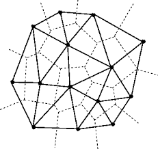
Figure 1: Delaunay (solid lines) with overlay of its dual graph called the voronoi diagram (dashed lines)

Figure 2: 2D perturbations, normative, linear gradient, radial gradient, random reduction (from top to bottom) at two densities
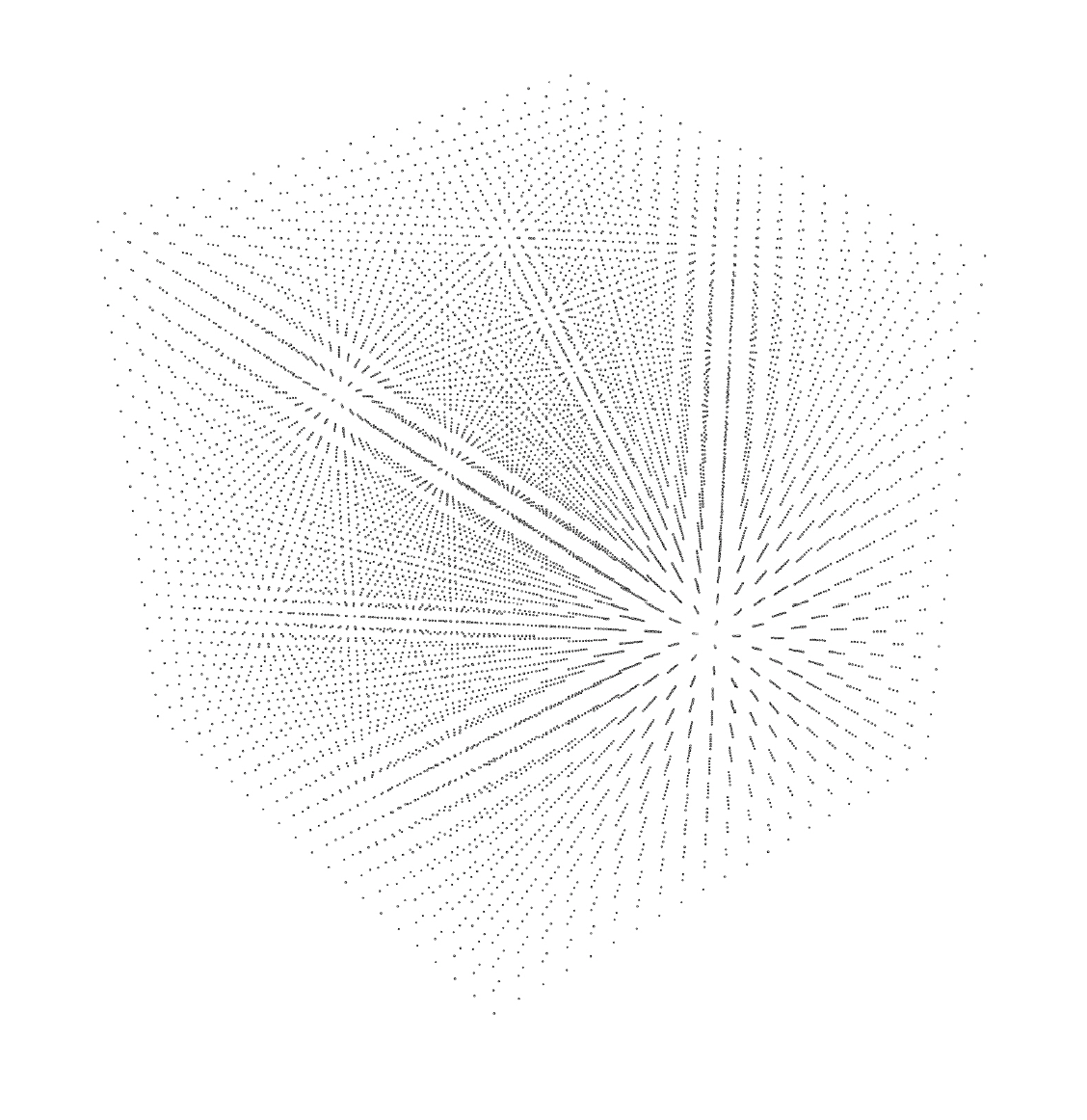
Figure 3 :3D array of unperturbed points
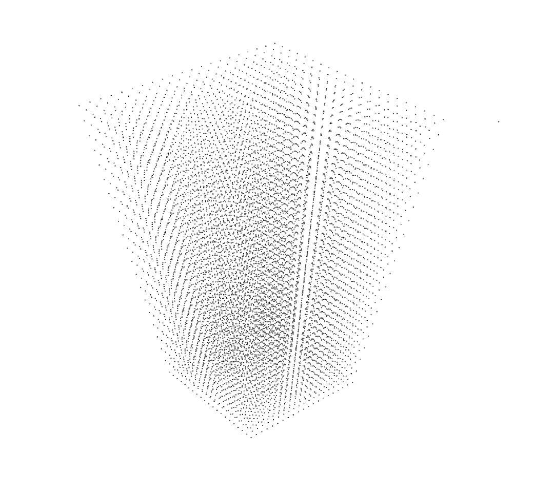
Figure 4: 3D array of points perturbed by ’tapering’
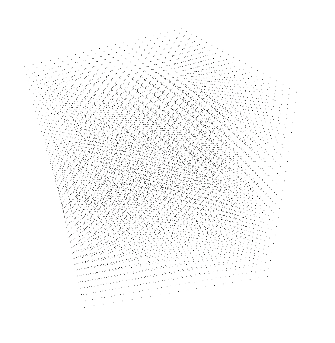
Figure 5: 3D array of points perturbed by ’twisting’

Figure 6:Connectivity (left) vs Proximity (right) on unperturbed networks

Figure 7: Connectivity (left) vs Proximity (right) on perturbed networks
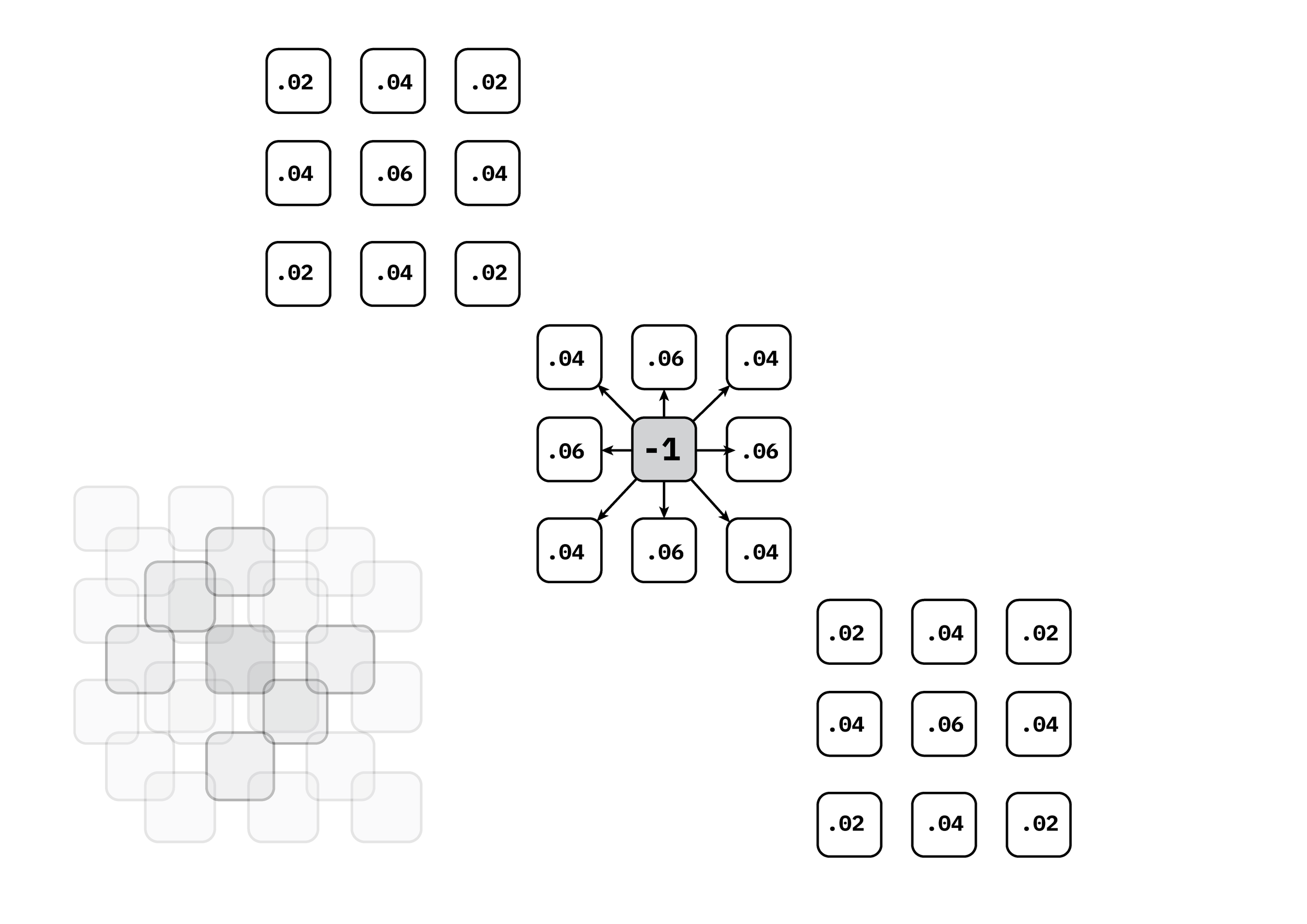
Figure 8: A 3D laplacian matrix with multiplier values broken out into 3 layers

Figure 9: An examples of iso-surfaces in a vector field
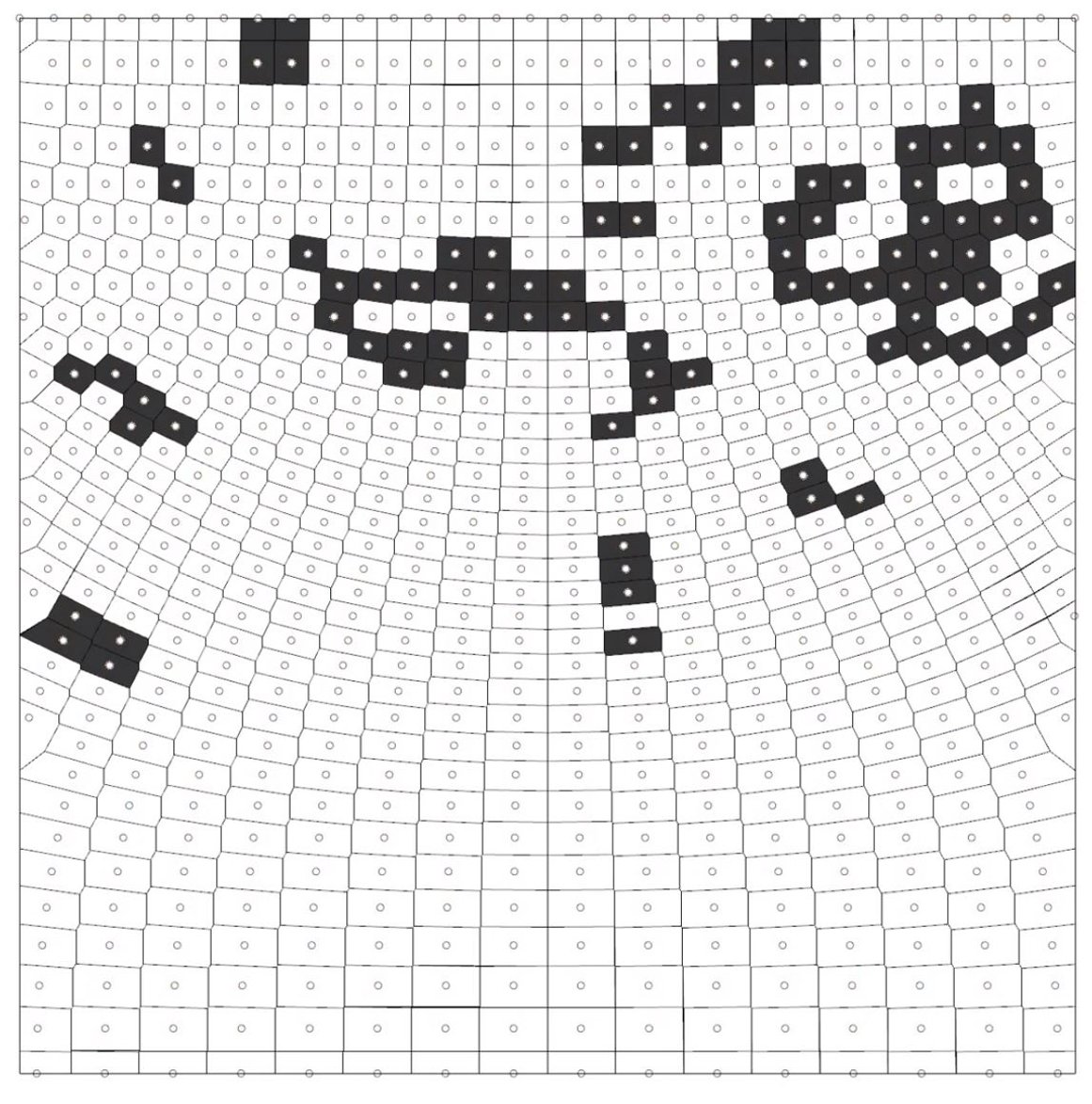
Figure 10: Frame from start of simulation
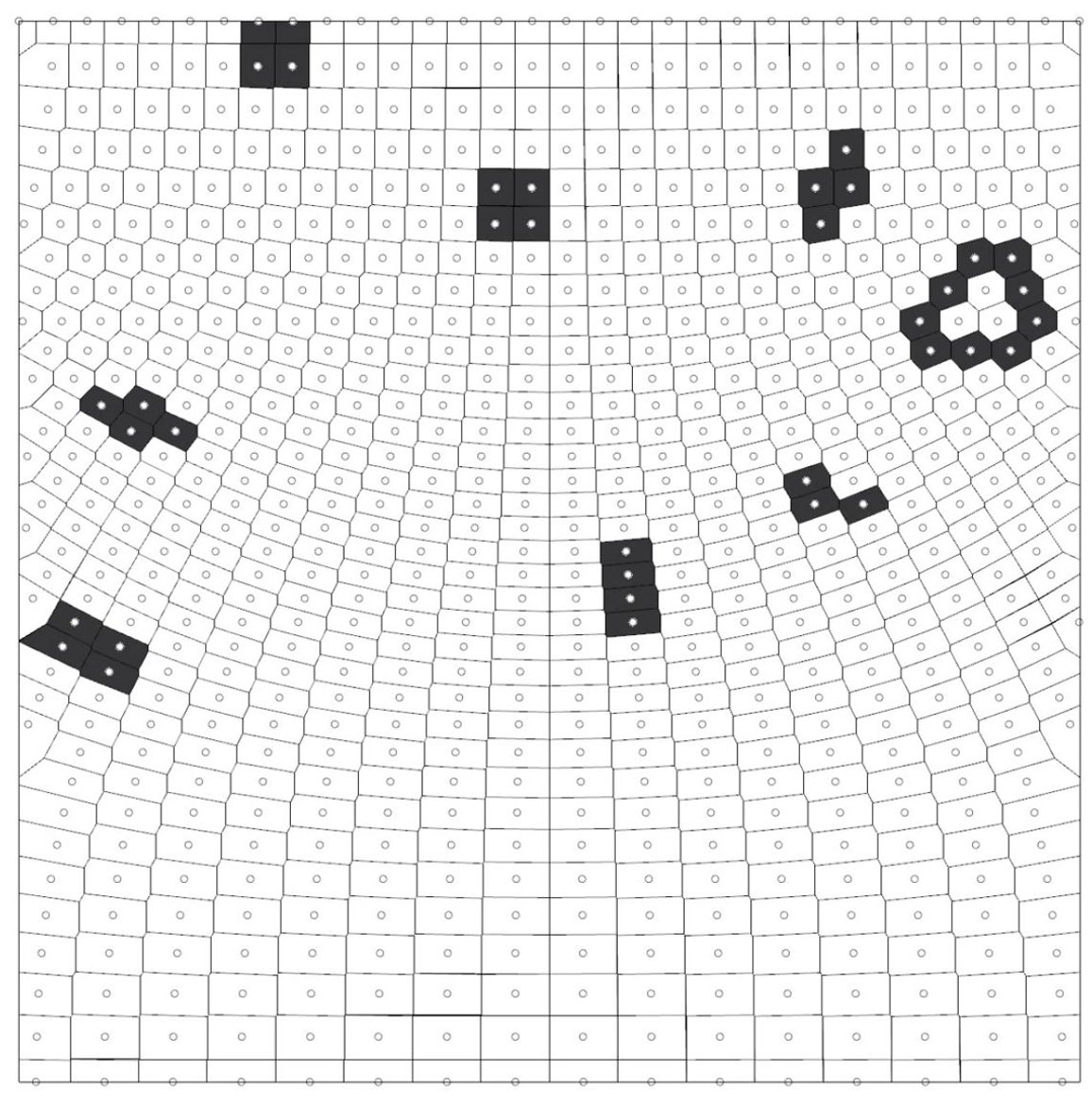
Figure 11: Converged simulation
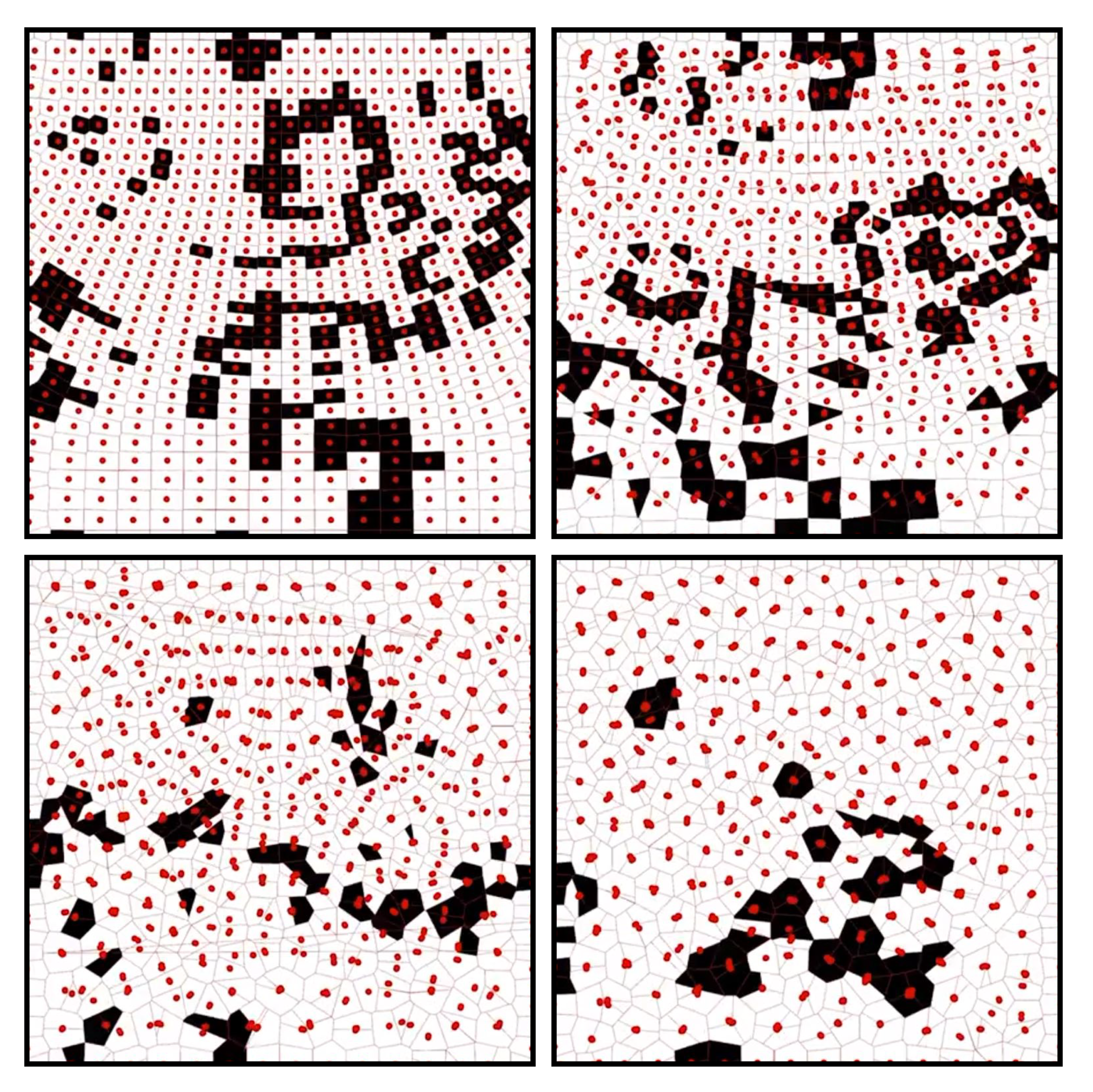
Figure 12: A series of states from the simulation showing the adaptive nodes returning a uniform distribution while propagating ’GoL’ activity

Figure 13: 3D GoL voronoi cells on perturbed points (top: twisted, bottomt: tapered)

Figure 14: 3D Reaction Diffusion with tapered perturbation of points at varying ratios

Figure 15: 3D Reaction Diffusion with twisted perturbation of points at varying angles